

XGBoost 관련 개념을 정리한 문서입니다. 논문을 보고 진행했어야 했는데 인터넷 자료를 바탕으로 작성하게 되었네요. 수식은 이해안되는 부분이 아직은 많아서 제외시켰습니다. 추후 논문을 확인해볼 생각입니다.
2022. 2. 22 최초작성
앙상블(Ensemble)
앙상블(Ensemble)은 여러 개의 모델을 사용해서 각각의 예측 결과를 만들고 그 예측 결과를 기반으로 최종 예측결과를 결정하는 방법입니다.
대표적인 예로 배깅(Bagging)과 부스팅(Boosting)이 있습니다.
베깅(Bagging)
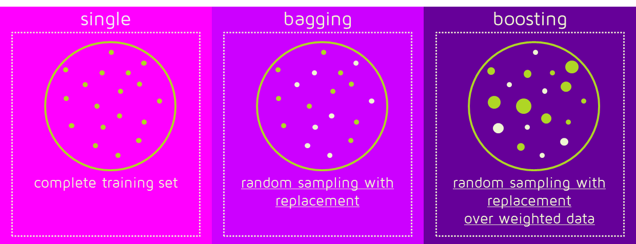
Bagging은 분할정복(divide and conquer and combine)과 같은 것입니다. 먼저 전체 훈련 데이터 세트를 여러개의 작은 샘플 훈련 데이터 세트로 나눕니다. 각각의 샘플 훈련데이터셋 별로 모델을 학습시킵니다. 마지막으로 모든 모델을 결합하여 전체 데이터 세트에 대한 최적의 모델을 얻습니다. 모델을 결합하는 방법으로 평균, 가중 평균, 투표 등을 사용할 수 있습니다.
예) 랜덤 포레스트

배깅 방식은 여러 개의 모델이 독립적입니다. 여러 개의 모델을 만들지만 이 과정에서 각각의 모델들은 서로의 영향을 받지 않습니다. 여러 개의 모델을 만들기 위해 각 모델별로 임의의 데이터 세트를 생성하는데 이 때 복원 추출(하나를 뽑을때마다 뽑은걸 다시 넣어서 다음번 뽑을때 다시 후보가 될 수 있게함)을 사용하여 무작위로 N개를 선택하여 데이터 세트를 생성합니다.
배깅 방식에서 만들어진 앙상블 모델을 이용해 예측을 실행할 때는 전체 모델의 평균을 계산(회귀 모델)하거나 과반수 투표를 실시(분류 모델)합니다.
배깅 방식의 대표적인 앙상블 모델은 랜덤 포레스트(Random Forest)입니다.
사이킷런 랜덤 포레스트 예제: https://baek2sm.blog.me/221768005852
부스팅(Boosting)
부스팅(Boosting)은 순차적으로 약한 학습자를 추가 결합하여 하나의 강한 모델 만드는 방법 입니다.
배깅과 마찬가지로 복원 추출을 사용하는데 샘플에 가중치를 부여하는 차이가 있습니다.
새로운 약한 학습자를 훈련시킬때 바로 전 약한 학습자의 학습결과에서 잘못 예측된 샘플에 대한 가중치는 증가시키고 올바르게 예측된 샘플에 대한 가중치는 감소시켜서 사용합니다.

이미지 출처
https://en.wikipedia.org/wiki/Boosting_(machine_learning)#/media/File:Ensemble_Boosting.svg
새로운 모델이 추가될때마다 오류 최소화를 목표로 학습됩니다. 이때마다 실제 값과 예측 값 사이의 오류를 계산합니다. 다음 그림처럼 모델이 추가됨에 따라 예측 오류가 줄어들게 됩니다.

Boosting을 사용하는 대표적인 모델은 AdaBoost, Gradient Boosting 등이 있고 XGBoost는 그 중 Gradient를 이용하여 Boosting하는 Gradient Boosting 을 사용해서 모델링을 합니다.
부스팅 방식의 대표적인 앙상블 모델은 그래디언트 부스팅(Gradient Boosting)입니다.
사이킷런 그래디언트 부스팅 예제: https://baek2sm.blog.me/221769091385
그라디언트 부스팅(Gradient Boosting)
그라디언트 부스팅(Gradient Boosting) = 경사하강법(Gradient Descent) + 부스팅(Boosting)
경사하강법(Gradient Descent)은 주어진 함수의 극소값을 찾는 데 사용되는 최적화 알고리즘입니다.
기본 개념은 주어진 함수의 기울기를 구하고 기울기의 절댓값이 낮은 쪽으로 계속 이동하여 극소값에 이를 때까지 반복하는 것입니다.

이미지 출처 - http://uc-r.github.io/gbm_regression
약한 학습자가 결합하여 형성된 기존 트리의 손실을 최소화하기 위해 새로운 약한 학습자를 한번에 하나씩 추가하며 기존 트리는 변경하지 않습니다. XGBoost에서는 약한 학습자로 결정 트리를 사용합니다.
모든 가능한 트리를 만들어보는 것은 불가능하므로 하나씩 추가하는 그리드 방식을 사용하는 것입니다.
경사 하강법을 사용하여 모델의 손실이 줄어들게 되는(모델 손실의 그레디언트가 낮아지도록) 트리를 모델에 추가합니다.
손실이 허용 가능한 수준에 도달하거나 검증 데이터 세트에서 더 이상 개선되지 않으면 훈련이 중지됩니다.
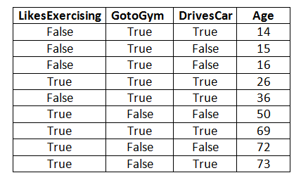
다음 예에서 Age는 Target 변수(=종속변수?)이고 LikesExercising, GotoGym, DrivesCar는 독립 변수입니다. 이 예에서와 같이 대상 변수는 연속적이며 여기에서는 GradientBoostingRegressor가 사용됩니다.
1st-Estimator
Estimator-1의 경우 루트 수준(수준 0)은 모든 레코드로 구성됩니다. 이 수준에서 예상 연령은 전체 연령 열의 평균, 즉 41.33과 같습니다(연령 열의 모든 값을 더한 값을 레코드 수로 나눈 값 즉, 9).
이 수준의 MSE가 무엇인지 알아보겠습니다. MSE는 오차 제곱의 평균으로 계산됩니다. 여기서 오류는 "실제 연령 - 예상 연령"과 같습니다. 특정 노드에 대한 예측 연령은 항상 해당 노드의 "연령 레코드의 평균"과 동일합니다. 따라서 1st estimator의 루트 노드의 MSE는 다음과 같이 계산됩니다.

여기서 비용 함수는 MSE이고 여기서 알고리즘의 목적은 MSE를 최소화하는 것입니다.
이제 독립 변수 중 하나가 결정 스텀프를 생성하기 위해 그라디언트 부스팅에 의해 사용됩니다. 여기서 LikesExercising이 예측에 사용된다고 가정해 보겠습니다. 따라서 False LikesExercising이 있는 레코드는 왼쪽 자식 노드로 이동하고 True LikesExercising이 있는 레코드는 아래와 같이 오른쪽 자식 노드로 이동합니다.
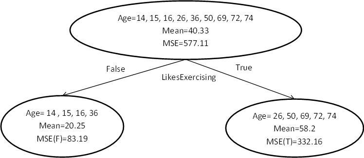
수준 1의 두 노드의 평균과 MSE를 계산해 보겠습니다. 왼쪽 노드의 경우 평균은 20.25이고 MSE는 83.19입니다. 반면 오른쪽 노드의 경우 평균은 58.2이고 MSE는 332.16입니다. 레벨 1의 총 MSE는 레벨 1의 모든 노드를 더한 것과 같습니다(예: 83.19+332.16=415.35). 여기에서 비용 함수, 즉 수준 1의 MSE가 수준 0보다 나은 것을 볼 수 있습니다.
2nd-Estimator:
Gradient boosting 알고리즘에서는 아래 그림과 같이 첫 번째 추정량의 나머지(age_i – mean)를 루트 노드로 사용합니다.
14 - 20.25 = -6.25
15 - 20.25 = -5.25
16 - 20.25 = -4.25
36 - 20.25 = 15.75
26-58.2 = -32.2
50-58.2 = -8.2
69 - 58.2 = 10.8
72 - 58.2 = 13.8
74 - 58.2 = 15.8
이 추정기에 대해 다른 종속 변수가 예측에 사용된다고 가정해 보겠습니다. 따라서 False GotoGym이 있는 레코드는 왼쪽 자식 노드로 이동하고 True GotoGym이 있는 레코드는 아래와 같이 오른쪽 자식 노드로 이동합니다.

여기서 나이 예측은 약간 까다롭습니다. 먼저 LikeExercising의 값에 따라 estimator1에서 나이를 예측하고 GotoGym의 값을 이용하여 estimator의 평균을 구하고 첫 번째 estimator에서 예측한 나이에 그 평균을 더하고 이것이 두 개의 추정기를 사용한 그라디언트 부스팅의 최종 예측입니다.
다음 레코드의 나이를 예측하려는 경우를 고려해 보겠습니다.

1차 추정기에서 LikesExercising는 False이므로 첫 번째 추정기의 예측 연령은 20.25세(즉, 첫 번째 추정기의 왼쪽 노드 평균)가 됩니다.
2차 추정기에서 GotoGym은 True이므로 두번째 추정기의 예측 연령은 -3.56세입니다.(즉, 두번째 추정기의 오른쪽 노드 평균)
1차 추정기의 예측 연령에 2차 추정기의 예측 연령을 더합니다. 따라서 이 모델의 최종 예측은 20.25+(-3.56) = 16.69가 됩니다.
예제에 있는 모든 레코드의 나이를 예측해 보겠습니다.

이제 모든 9개 레코드에 대한 최종 MSE를 알아보겠습니다.

따라서 최종 MSE가 1st Estimator 루트 노드의 MSE보다 훨씬 우수함을 알 수 있습니다. 이것은 2명의 추정자에게만 해당됩니다. 그래디언트 부스팅 알고리즘에는 n개의 추정기가 있을 수 있습니다.
앞에서 설명한 내용을 코드로 작성한 예시라는데 결과만 확인해보고 아직 분석을 해보기 전입니다.
import pandas as pd
from sklearn.ensemble import GradientBoostingRegressor
from sklearn.preprocessing import LabelEncoder
X=pd.DataFrame({'LikesExercising':[False,False,False,True,False,True,True,True,True],
'GotoGym':[True,True,True,True,True,False,True,False,False],
'DrivesCar':[True,False,False,True,True,False,True,False,True]})
Y=pd.Series(name='Age',data=[14,15,16,26,36,50,69,72,74])
# Let us encode true and false to number value 0 and 1
LE=LabelEncoder()
X['LikesExercising']=LE.fit_transform(X['LikesExercising'])
X['GotoGym']=LE.fit_transform(X['GotoGym'])
X['DrivesCar']=LE.fit_transform(X['DrivesCar'])
#We will now see the effect of different numbers of estimators on MSE.
# 1) Let us now use GradientBoostingRegressor with 2 estimators to train the model and to predict the age for the same inputs.
GB=GradientBoostingRegressor(n_estimators=2)
GB.fit(X,Y)
Y_predict=GB.predict(X) #ages predicted by model with 2 estimators
print('two estimators')
print(Y_predict)
# Output
#Y_predict=[38.23 , 36.425, 36.425, 42.505, 38.23 , 45.07 , 42.505, 45.07 ,47.54]
#Following code is used to find out MSE of prediction with Gradient boosting algorithm having estimator 2.
MSE_2=(sum((Y-Y_predict)**2))/len(Y)
print('MSE for two estimators :',MSE_2)
#Output: MSE for two estimators : 432.482055555546
print('\n\n')
# 2) Let us now use GradientBoostingRegressor with 3 estimators to train the model and to predict the age for the same inputs.
GB=GradientBoostingRegressor(n_estimators=3)
GB.fit(X,Y)
Y_predict=GB.predict(X) #ages predicted by model with 3 estimators
print('three estimators')
print(Y_predict)
# Output
#Y_predict=[36.907, 34.3325, 34.3325, 43.0045, 36.907 , 46.663 , 43.0045, 46.663 , 50.186]
#Following code is used to find out MSE of prediction with Gradient boosting algorithm having estimator 3.
MSE_3=(sum((Y-Y_predict)**2))/len(Y)
print('MSE for three estimators :',MSE_3)
#Output: MSE for three estimators : 380.05602055555556
print('\n\n')
# 3) Let us now use GradientBoostingRegressor with 50 estimators to train the model and to predict the age for the same inputs.
GB=GradientBoostingRegressor(n_estimators=50)
GB.fit(X,Y)
Y_predict=GB.predict(X) #ages predicted by model with 50 estimators
print('fifty estimators')
print(Y_predict)
# Output
#Y_predict=[25.08417833, 15.63313919, 15.63313919, 47.46821839, 25.08417833, 60.89864242, 47.46821839, 60.89864242, 73.83164334]
#Following code is used to find out MSE of prediction with Gradient boosting algorithm having estimator 50.
MSE_50=(sum((Y-Y_predict)**2))/len(Y)
print('MSE for fifty estimators :',MSE_50)
#Output: MSE for fifty estimators: 156.5667260994211
GridSearchCV를 사용한 최적 모델을 찾는 예제입니다. 아직 분석 전이며 결과 개선만 해봤습니다.
import numpy as np
import pandas as pd
from sklearn.ensemble import GradientBoostingRegressor
from sklearn.preprocessing import LabelEncoder
from sklearn.experimental import enable_halving_search_cv # HalvingRandomSearchCV 임포트시 필요
from sklearn.model_selection import GridSearchCV, HalvingRandomSearchCV
X=pd.DataFrame({'LikesExercising':[False,False,False,True,False,True,True,True,True],
'GotoGym':[True,True,True,True,True,False,True,False,False],
'DrivesCar':[True,False,False,True,True,False,True,False,True]})
Y=pd.Series(name='Age',data=[14,15,16,26,36,50,69,72,74])
# Let us encode true and false to number value 0 and 1
LE=LabelEncoder()
X['LikesExercising']=LE.fit_transform(X['LikesExercising'])
X['GotoGym']=LE.fit_transform(X['GotoGym'])
X['DrivesCar']=LE.fit_transform(X['DrivesCar'])
model=GradientBoostingRegressor()
params={'n_estimators':range(1,200)}
grid=GridSearchCV(estimator=model,cv=2,param_grid=params,scoring='neg_mean_squared_error')
grid.fit(X,Y)
print("The best estimator returned by GridSearch CV is:",grid.best_estimator_)
#Output
#The best estimator returned by GridSearch CV is: GradientBoostingRegressor(n_estimators=19)
GB=grid.best_estimator_
GB.fit(X,Y)
Y_predict=GB.predict(X)
Y_predict
#output:
#Y_predict=[27.20639114, 18.98970027, 18.98970027, 46.66697477, 27.20639114,58.34332496, 46.66697477, 58.34332496, 69.58721772]
MSE_best=(sum((Y-Y_predict)**2))/len(Y)
print('MSE for best estimators :',MSE_best)
#Following code is used to find out MSE of prediction for Gradient boosting algorithm with best estimator value given by GridSearchCV
#Output: MSE for best estimators : 164.2298548605391
#Observation:
# n_estimator=50에 대한 MSE가 n_estimator=19에 대한 MSE보다 낫다고 생각할 수 있습니다.
# 하지만 GridSearchCV는 50이 아닌 19를 반환합니다.
# 실제로, 추정값이 증가할 때마다 MSE의 감소가 상당하는 것은 19까지임을 관찰할 수 있습니다.
# 19 이후에는 추정량이 증가해도 MSE가 크게 감소하지 않습니다.
# 따라서 n_estimator=19가 GridSearchCV에서 반환되었습니다.
# HalvingRandomSearchCV라는 다른 방법을 적용해봤습니다.
model=GradientBoostingRegressor()
param_grid = {
'learning_rate': list(np.linspace(0.001, 0.1, 20)),
'n_estimators': list(np.arange(1, 200)),
#'subsample': list(np.linspace(0.4, 1, 20)),
'max_depth': list(np.linspace(1, 12, 12, dtype=int))
}
grid=HalvingRandomSearchCV(estimator=model,cv=2,param_distributions=param_grid,scoring='neg_mean_squared_error')
grid.fit(X,Y)
print("The best estimator returned by HalvingRandomSearchCV is:",grid.best_estimator_)
#Output
#The best estimator returned by GridSearch CV is: GradientBoostingRegressor(n_estimators=19)
GB=grid.best_estimator_
GB.fit(X,Y)
Y_predict=GB.predict(X)
Y_predict
#output:
#Y_predict=[27.20639114, 18.98970027, 18.98970027, 46.66697477, 27.20639114,58.34332496, 46.66697477, 58.34332496, 69.58721772]
MSE_best=(sum((Y-Y_predict)**2))/len(Y)
print('MSE for best estimators :',MSE_best)
실행 결과입니다. 앞에서 언급한 것처럼 GridSearch CV는 최적값을 찾기전 중단되는데 반해 HalvingRandomSearchCV는 최적값에 가까운 값을 찾아줍니다.
The best estimator returned by GridSearch CV is: GradientBoostingRegressor(n_estimators=19)
MSE for best estimators : 164.2298548605391
The best estimator returned by HalvingRandomSearchCV is: GradientBoostingRegressor(learning_rate=0.03226315789473684, n_estimators=142)
MSE for best estimators : 156.593477404869
결정트리(Decision Tree)
결정 트리(Decision Tree)는 샘플을 분류하기 위해 반복적으로 질문을 하는 방식입니다.
내부 노드에서 속성에 대한 질문을 하여 분기로 질문에 대한 답변 결과를 나누며, 각 리프 노드가 클래스 레이블을 의미하는 트리 구조입니다.

이미지 출처 - https://ko.wikipedia.org/wiki/결정_트리_학습법
타이타닉호 탑승객의 생존 여부를 나타내는 결정 트리입니다. 리프 노드에 있는 두개의 숫자는 각각 생존 확률과 탑승객이 그 리프 노드에 해당될 확률을 의미합니다.
XGBoost
XGBoost(eXtreme Gradient Boosting)는 그레디언트 부스트 결정 트리(Gradient Boosted Decision Trees) 알고리즘의 오픈 소스 구현입니다.
XGBoost는 분류(Classification), 회귀(Regression) 등의 모델을 제공합니다.
XGBoost 라이브러리에도 자체 API가 있지만 사이킷런(scikit-learn) 래퍼 클래스인 XGBRegressor 및 XGBClassifier를 사용합니다. scikit-learn 라이브러리를 사용하여 데이터를 준비하고 모델을 평가하기 위해서 입니다.
XGBRegressor는 Regression을 위한 XGBoost 모델이며 XGBClassifier는 Classification을 위한 XGBoost Model입니다.
결정 트리 앙상블(Decision Tree Ensembles)
결정 트리 앙상블(decision tree ensembles) 중 하나가 XGBoost의 기반 모델인 gradient boosting decision trees (GBDT)이다.
결정 트리 앙상블 모델은 Classification And Regression Tree(CART)로 구성됩니다.
CART는 Decision Tree를 생성하는 대표적인 알고리즘으로 분류와 회귀에 모두 사용가능합니다.
CART 예시)
누가 가상의 컴퓨터 게임 X를 좋아하는지를 질문을 통해 분류하는 CART의 간단한 예

컴퓨터 게임 X를 좋아하는지 알아보기 위해 조건으로 나이가 20살 미만인지 체크하여 맞다면 가산점 2를 주고 틀리다면 감점 1을 줍니다.
조건을 만족하는지 여부에 따라 가족 구성원을 다른 리프(leaf)로 분류하고 속한 리프에 따라 다른 점수(score)를 할당합니다.
일반적으로 단일 트리는 실제로 사용하기에 충분히 강하지 않습니다. 실제로 사용되는 것은 여러 트리의 예측을 결합하는 앙상블 모델입니다.
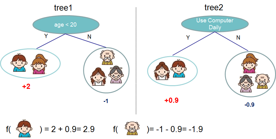
첫번째 경우는 나이가 20살 미만이고 매일 컴퓨터를 사용하므로 둘다 가산점을 받아서 2 + 0.9 = 2.9가 됩니다.
두번째 경우는 나이가 20살 이상이고 매일 컴퓨터를 사용하지 않으므로 둘다 감점을 받아서 -1-0.9=-1.9가 됩니다.
두 개의 트리의 예측을 결합하여 샘플에 대한 최종 점수를 얻었습니다. 그 결과 첫번째 사람이 두번째 사람보다 게임을 좋아할 가능성이 높은것으로 예측됩니다.
참고
https://ssoonidev.tistory.com/106
https://xgboost.readthedocs.io/en/stable/tutorials/model.html
https://neptune.ai/blog/gradient-boosted-decision-trees-guide
https://www.geeksforgeeks.org/xgboost/
https://medium.com/@6453gobind/gradient-boosting-15ecc572a988
https://en.wikipedia.org/wiki/Boosting_(machine_learning)
https://www.kdnuggets.com/2019/09/ensemble-learning.html
https://exupery-1.tistory.com/183
https://gentlej90.tistory.com/100
https://gentlej90.tistory.com/87
https://www.ccs.neu.edu/home/vip/teach/MLcourse/4_boosting/slides/gradient_boosting.pdf
https://ko.wikipedia.org/wiki/경사_하강법
https://towardsdatascience.com/gradient-descent-algorithm-a-deep-dive-cf04e8115f21
https://blog.paperspace.com/gradient-boosting-for-classification/
https://exupery-1.tistory.com/182
https://m.blog.naver.com/baek2sm/221771893509
https://machinelearningmastery.com/gentle-introduction-gradient-boosting-algorithm-machine-learning/
https://www.analyticsvidhya.com/blog/2021/04/how-the-gradient-boosting-algorithm-works/
http://machinelearningkorea.com/2019/09/28/xgboost-논문따라가기/
'Deep Learning & Machine Learning > 딥러닝&머신러닝 개념' 카테고리의 다른 글
| 기대값이란 (0) | 2023.11.05 |
|---|---|
| 신경망(neural networks)에서 편향(bais)의 역할 (0) | 2023.10.28 |
| 정규화(Normalization), 표준화(standardization), 이상치(outlier) 제거 (0) | 2023.10.23 |
| 난수 생성에서 시드(seed) 사용하는 이유 (0) | 2023.10.12 |
| 분산과 표준 편차 차이 정리 (2) | 2023.10.09 |
시간날때마다 틈틈이 이것저것 해보며 블로그에 글을 남깁니다.
블로그의 문서는 종종 최신 버전으로 업데이트됩니다.
여유 시간이 날때 진행하는 거라 언제 진행될지는 알 수 없습니다.
블로그 글과 유튜브 영상을 만드는 것은 전문가라서라기보단 공부한 내용을 함께 공유하는 게 좋아서입니다.
제가 쓴 책도 한번 검토해보세요 ^^


#/media/File:Ensemble_Boosting.svg)