
Matplotlib로 FFT 그려보기Python/Matplotlib2022. 1. 17. 18:06
Table of Contents
반응형
Matplotlib를 사용하여 FFT를 그려보았습니다.
2021. 12. 18 최초작성
2021. 12. 31 예제 코드 추가
2021. 01. 17 예제 코드 추가
아직 정확히 개념이 잡힌 상태가 아니라서 틀린점이 있을 수 있으니 참고용으로만 사용하세요.
다음 두 개의 sin 그래프를 FFT로 변환하여 그려봅니다.
오른쪽의 진폭이 2배 더 큽니다.

왼쪽은 FFT로 변환한 결과이며 오른쪽은 FFT 결과를 역변환하여 얻은 원래 파형을 그린것입니다.
두 개의 sin 그래프의 FFT 결과에서 다른 점은 1Hz에서의 높이가 원래 파형의 배수만큼 다른 것입니다.
원래 그래프에서 2배 차이가 났었는데 FFT의 1Hz에서의 높이도 2배 차이입니다.

전체 소스코드입니다.
# 참고 : https://pythonnumericalmethods.berkeley.edu/notebooks/chapter24.04-FFT-in-Python.html import numpy as np from matplotlib import pyplot as plt from numpy.fft import fft, ifft x = np.arange(0, 60) y1 = np.sin(7*x * np.pi / 180. ) y2 = np.sin(7*x * np.pi / 180. + 3 ) * 2 plt.figure(figsize = (12, 6)) plt.subplot(121) plt.plot(x, y1, color='r') plt.subplot(122) plt.plot(x, y2, color='b') plt.show() data = [y1, y2] for d in data: x = d sr = 60 # sampling rate ts = 1.0/sr # sampling interval t = np.arange(0, 1, ts) X = fft(x) N = len(X) n = np.arange(N) T = N/sr freq = n/T plt.figure(figsize = (12, 6)) plt.subplot(121) plt.stem(freq, np.abs(X), 'b', markerfmt=" ", basefmt="-b") plt.xlabel('Freq (Hz)') plt.ylabel('FFT Amplitude |X(freq)|') plt.xlim(0, 10) plt.subplot(122) plt.plot(t, ifft(X), 'r') plt.xlabel('Time (s)') plt.ylabel('Amplitude') plt.tight_layout() plt.show() |
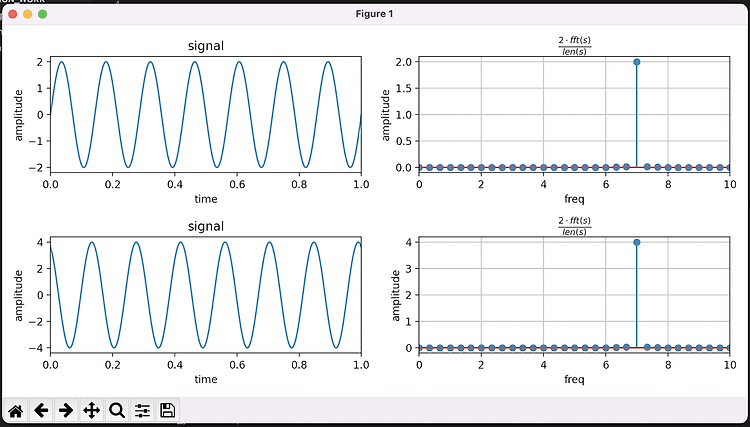
sine 파를 생성할 때 주파수로 7 Hz를 사용하였더니 FFT 결과 7 HZ 위치에만 값이 존재합니다.

전체 코드입니다.
| # 참고 # https://tuttozurich.tistory.com/15 # https://github.com/hazevt04/fft_sine_wave/blob/main/fft_sine_wave.py import numpy as np from matplotlib import pyplot as plt freq = 7 # Frequency of the Sinewave rate = 1000 # Sampling Rate time_interval = 3 # Sampling Interval t = np.linspace(0, time_interval, time_interval*rate) # Time-Axis y1 = 2*np.sin(2*np.pi*freq*t) # Sinewave y2 = 4*np.sin(2*np.pi*freq*t + 2) # Sinewave def PositiveFFT(x, Fs): Ts = 1/Fs Nsamp = x.size xFreq = np.fft.rfftfreq(Nsamp, Ts)[:-1] yFFT = (np.fft.rfft(x)/Nsamp)[:-1]*2 return xFreq, yFFT # Calculate FFT xFreq1, FFT_data1 = PositiveFFT(y1, rate) xFreq2, FFT_data2 = PositiveFFT(y2, rate) # Plot the FFT fig, ((ax1, ax2), (ax3, ax4)) = plt.subplots(2, 2, figsize = (10,5)) ax1.plot(t, y1) ax1.set_title('signal') ax1.set_xlabel('time') ax1.set_ylabel('amplitude') ax1.set_xlim(0,1) ax2.stem(xFreq1, abs(FFT_data1), use_line_collection=True) ax2.grid(True) ax2.set_title(r"$\frac{2 \cdot fft(s)}{len(s)}$") ax2.set_xlabel('freq') ax2.set_ylabel('amplitude') ax2.set_xlim(0,10) ax3.plot(t, y2) ax3.set_title('signal') ax3.set_xlabel('time') ax3.set_ylabel('amplitude') ax3.set_xlim(0,1) ax4.stem(xFreq2, abs(FFT_data2), use_line_collection=True) ax4.grid(True) ax4.set_title(r"$\frac{2 \cdot fft(s)}{len(s)}$") ax4.set_xlabel('freq') ax4.set_ylabel('amplitude') ax4.set_xlim(0,10) plt.tight_layout() plt.show() |
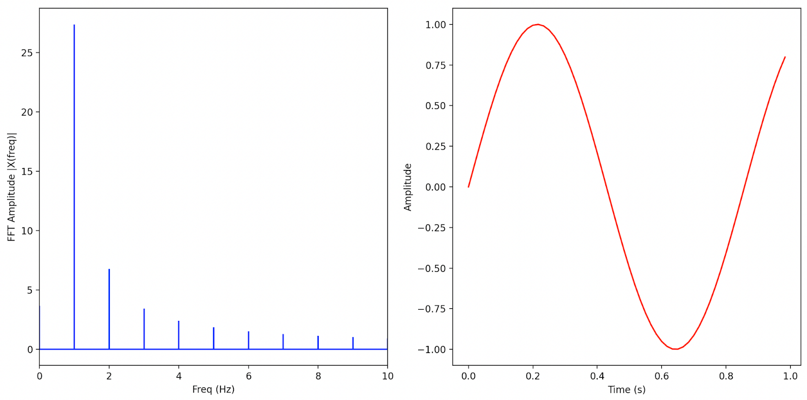
5 Hz, 7 Hz, 9 Hz 사인파를 더한 후, FFT 변환하여 스펙트럼을 그려보았습니다. 사인파를 위한 주파수별로 성분이 검출되었습니다.

| # 참고 # https://tuttozurich.tistory.com/15 # https://github.com/hazevt04/fft_sine_wave/blob/main/fft_sine_wave.py # https://alice-secreta.tistory.com/22 # https://techreviewtips.blogspot.com/2017/11/05-02-fft.html import numpy as np from matplotlib import pyplot as plt freq1 = 5 # Frequency of the Sinewave 5 Hz freq2= 7 # 7 Hz freq3 = 9 # 9 Hz Fs = 1000 # Sampling Rate time_interval = 1 # Sampling Interval t = np.arange(0, time_interval, 1/Fs) # 5Hz에 진폭이 2인 시그널을 1초동안 샘플링한다. y1 = 2*np.cos(2*np.pi*freq1*t) # Sinewave y1 += 2*np.cos(2*np.pi*freq2*t) # Sinewave y1 += 2*np.cos(2*np.pi*freq3*t) # Sinewave def PositiveFFT(x, Fs): Ts = 1/Fs Nsamp = x.size xFreq = np.fft.rfftfreq(Nsamp, Ts)[:-1] yFFT = (np.fft.rfft(x)/Nsamp)[:-1]*2 # yFFT = (np.fft.fft(x)/Nsamp) # yFFT = np.abs(yFFT[:int(Nsamp/2)])*2# 두배를 해야 하는가? # xFreq = np.fft.fftfreq(Nsamp, Ts)[:int(Nsamp/2)] return xFreq, yFFT # Calculate FFT xFreq1, FFT_data1 = PositiveFFT(y1, Fs) print(y1.shape, FFT_data1.shape) # Plot the FFT fig, (ax1, ax2) = plt.subplots(1, 2, figsize = (10,5)) ax1.plot(t, y1) ax1.set_title('signal') ax1.set_xlabel('time') ax1.set_ylabel('amplitude') ax1.set_xlim(0,1) ax2.stem(xFreq1, abs(FFT_data1), use_line_collection=True) ax2.grid(True) ax2.set_title(r"$\frac{2 \cdot fft(s)}{len(s)}$") ax2.set_xlabel('freq') ax2.set_ylabel('amplitude') ax2.set_xlim(0,10) plt.tight_layout() plt.show() |
반응형
'Python > Matplotlib' 카테고리의 다른 글
| Matplotlib 예제 – 하나의 figure에 여러 개의 이미지 출력하기 (0) | 2023.10.07 |
|---|---|
| Matplotlib 그래프에 라벨 추가하기 (0) | 2022.06.19 |
| for문으로 실행하여 Matplotlib 그래프 저장하는 예제 (0) | 2021.11.29 |
| Matplotlib에서 수직선 그리기 (0) | 2021.11.28 |
| Matplotlib에서 x축 눈금 레이블을 대각선으로 출력하기 (0) | 2021.10.28 |
시간날때마다 틈틈이 이것저것 해보며 블로그에 글을 남깁니다.
블로그의 문서는 종종 최신 버전으로 업데이트됩니다.
여유 시간이 날때 진행하는 거라 언제 진행될지는 알 수 없습니다.
영화,책, 생각등을 올리는 블로그도 운영하고 있습니다.
https://freewriting2024.tistory.com
제가 쓴 책도 한번 검토해보세요 ^^